Extraction and Modelling of Spatio-Temporal Urban Change in Kathmandu Valley

ABSTRACT

Urbanization is the continuous and complex ecological process arising various environmental and socio- economic issues of global change. In this study, the spatio- temporal urban growth rate and pattern of Kathmandu, Nepal were detected from 1989 to 2009 and by using the existing trend and factors of urban growth, simulation of urbanization is also prepared for the year of 2015, 2020, 2025, 2030 and 2035. Landsat TM imagery of four different year of Kathmandu valley is used to extract built up and non-built up area of the valley by using the supervised classification of remote sensing technique. Spatial metrics of three landscapes at three levels (patch, class, and landscape) were calculated using classified map as the input layer. These metrics were used to quantify the existing built up at different scale of patch, class and landscape which was used for further analysis of growth rate and pattern detection. The changing trend of these urban areas is now linked with the physical driving factors of urban growth and SLEUTH model were run to predict the future scenario of urbanization for the year of 2020, 2025, 2030, and 2035. The result of the model suggests that still the infill expansion will be occurred at the edge of the city forming more dense urbanization. Infill expansion is seen mostly in the center and the southern part of the city. Road influenced growth is seen mostly in the northern and the eastern part of the city forming many cities, towns and urban centers. Up to 2020, center of the city seems to saturate for urbanization leading rapid edge and road influenced expansion in northern part of the city up to 2030. But after 2030 model predicts that there will be slow urban growth of the valley. SLEUTH model used in this study can’t consider all the factors which also play an important role in the urban growth and neither incorporate various plans, accidents, policies and situations that may come in the near future, which may drastically change the pattern of urbanization as well. But, the prediction of this model can provide the most possible scenario of urbanization based on the trend of past and present, which can be used for informed decision making tool for policy formulation and planning sustainable & managed human habitat in Kathmandu.

Keywords

Remote Sensing, Image Classification, Spatial metrics,

Urban Growth Prediction Model, SLEUTH model

1. INTRODUCTION

Urbanization is a continuous and complex ecological phenomenon of increase in spatial extent and population of the urban areas (Cohen, 2006). In recent few decades urbanization and urban growth have gained the maximum acceleration all around the world and especially affecting the developing countries (Annez & Buckley, 2009). According to United Nations (United Nations, 2014), in

2014, 54 per cent of the world’s population was urban and the urban population is expected to continue to grow, so that by 2050, the world will be one third rural (34 per cent) and two-thirds urban (66 per cent) (Fig. 1).

Fig. 1. Urban and rural population of the world, 1950–

2050 (United Nations, 2014)

Urban system is very complex system and the factors affecting the urbanization are also dynamic in spatial, temporal and socio-economic dimension (Abd-Allah,

2007). In most developing countries, urbanization is

regarded as the crucial phenomenon of economic growth and social change as it offers the increase in opportunities for employment, specialization, better education, production, goods and services. This not only provides good opportunities, but, also triggers numerous problems (UN-Habitat, 2011). If not managed properly, these may intimidate sustainable development of cities in the long run ( Dubovyk et al., 2011).

Recent concerns on the sustainable development have nurtured a new interest on the physical dimension of the cities and mainly on the issues of urban growth pattern and urban form (Huang et al., 2007; Van de Voorde et al.,

2009). Numerous studies have been conducted focusing the phenomenon of urban sprawl and informal settlement and their adverse environmental and socio-economic consequences (Dubovyk et al., 2011; Schneider & Woodcock, 2008). Numerous researches such as (Bhatta,

2009; Clarke & Gaydos, 1998; Jat et al., 2008; Ji et al.,

2006; Sudhira et al., 2004; Xiao et al., 2006) have used combined approach of GIS and RS at different parts of the world as an application in urban growth detection, monitoring, factor determination, accuracy assessment and modeling for the future urban development of the city.

Urbanization has also been observed in Nepal form 1970s onward, showing on of the highest rate in Asia and the Pacific (ADB/ICIMOD, 2006). With a population of 2.5 million people, Kathmandu valley is growing by 4 percent per year and has become the most populated city in country as well one of the fastest growing metropolitan in South Asia (Muzzini & Aparicio, 2013). As the growth is very rapid and haphazard, understanding the urban growth pattern in valley will help local and regional planners to better understand the future demands of basic amenities like water, electricity, land utilization, sanitation and other facilities for planning and proper decision making.

The general objectives of this study are to detect and quantify the spatial-temporal trends and patterns of urban growth in Kathmandu valley from 1989 to 2014 using satellite image, remote sensing technique, GIS and spatial metrics. Furthermore, the study forecasts the urban growth of the study area using SLEUTH model from 2015 to

2035.

2. STUDY AREA AND DATA

Kathmandu; the capital city of Nepal, lies within 27° 32' 00" N to 27° 49'16" N latitude, 85°13'28" E to 85°31'53" E longitude and an elevation of approximately 1,400 meters. Half of the area has less than 5° slope; while more than 20% of land has greater than 20°. The city lies on the warm temperature zone having elevation range from 1,200-2,300 meters and the average temperature of the city varies from 28-30° C and average winter temperature of 10.1° C. the average rainfall for the city is measured to be 1,207mm and the average humidity of 75% (climate data for Kathmandu 1981-2010).

Politically, the valley comprises of five municipal urban centers (Kathmandu, Lalitpur, Bhaktapur, Kritipur and Madyapur Thimi) with addition of 97 surrounding villages. According to a census conducted in 2011, Kathmandu metropolis alone has 975,453 inhabitants; and the agglomerate has a population of more than 2.5 million inhabitants. The metropolitan city area is 684 square kilometers with the 14% of the land with urban centers and has a population density of 129,250 per km²(CBS, 2012). As it is the capital city of the country, it is well facilitated than the other part of the country in terms of educational and health institution, communication and transportation facility.

Fig. 2. Location map of the study area

In this study, multi-temporal scenes of satellite images and various thematic and topographic maps were used as input. Freely available various data layers: Kathmandu boundary, contour, spot heights, river, road and landuse (1978 and

1995), produced by the ICIMOD (http://www.icimod.org/) were collected from its data portal for the study. Landsat TM images of 1989, 1999, 2009 and 2014 were obtained from the United States Geological Survey (USGS) (http://glovis.usgs.gov/) in the standard TIFF format, which were radio-metrically and geometrically correct. To avoid the seasonal variation, images were downloaded for nearly same seasonal time avoiding the cloud percentage as much as possible except of 2014. All images were form same row and path (141/011), same resolution (30 m), and same geographical extent. The properties of images are given in table1. The ground truth points used during the accuracy assessment of the image classification was acquired from the Digital Globe image using Google Earth software and field visit.

Table 1. Properties of images used for Image classification

image that represents the true spectral radiance at the sensor. With the help of the information (metadata) provided with the satellite imagery, ENVI’s radiometric calibration tool was used to calibrate images to radiance. As Kathmandu is the valley surrounded by the mountains,

Satellite

Sensor

Landsat

5 TM

Landsat

7 ETM+

Landsat

5 TM

Landsat

8 OLI

the effect of cast shadows of mountains present in the

satellite image may create the ambiguity among the

Date 1989-10-31 1999-11-04 2009-11-23 2014-03-26

Various software are used for this study: ENVI and ArcGIS for editing and mapping, FRAGSTATS for quantifying the landscape pattern and SLUETH model for urban growth prediction. Others program used for aid and basic function are Map Source, ExpertGPS, PC-Pine and Google Earth.

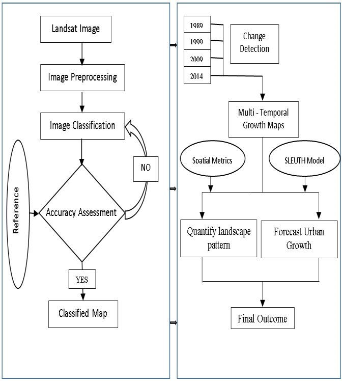
3. METHODOLOGY

In order to achieve the aims and objectives of the study, three major techniques namely Remote Sensing, Spatial Metrics and SLEUTH modeling were employed. Landsat Image downloading, preprocessing, signature extraction, image classification and accuracy assessment was done in remote sensing technique. Different metrics were used to quantify the landscape pattern in spatial metrics technique and modeling to forecast the urban growth was done in SLEUTH Model technique. The overall conceptual framework of the study adapted for the study is shown in the Fig. 3.

Fig. 3. Flow Diagram of overall methodology

A. Remote Sensing

First of all, pre-processing was done using ENVI 4.3 to

enhance data quality. The pre-processing tasks involved calibration, topographic correction and atmospheric correction of the image. Calibration was done to compensate for radiometric errors from sensor defects, variation in scan angle, and system noise to produce an

components of scene. So to remove such effects,

topographic correction was performed using cosine correction algorithm. Dark object subtraction method was employed in order to correct the atmospheric effects.

The method suggested by Xu (2007) was employed to classify the image into two classes namely built ups and non-built. Three images for built, water and vegetation were prepared and stacked. Using these three band image, Index-Based Images were prepared. Supervised image classification approach specifically maximum likelihood algorithm was used to prepare the binary image of built and non-built class.

In this study, accuracy assessment was checked creating confusion matrix. Confusion matrix was generated by the sampling approach in which the number of raster elements from the output class was selected and then both classification and true world classes were compared. This comparison was done by generating confusion matrix or error matrix. Out of various sampling schemes, samples required to determine the true accuracy of built-up class were collected. The number of samples to assure the quality of classification was determined by using sampling theory. Twenty samples covering the study area uniformly were selected to generate the error matrix.

Change detection was simply done by the difference between two images of consecutive years. The classified images were overlaid in the order 1989, 1999, 2009 and

2014 to visualize the direction of the growth via choropleth map. Rate of growth rate in terms of percentage and changed areas were also calculated.

B. Spatial Metrics

The classified images were used as input to calculate the spatial metrics in FRAGSTATS software to quantify the

urban landscape fragmentation process and patterns. Change in urban area were detected and hence quantified and then categorized them using spatial metrics to simple and identifiable patterns. Following metrics were computed to quantify the landscape pattern: Class area

(CA), Number of patches (NP), Patch Density (PD),

Largest Patch Index (LPI), Edge density(ED), Area Weighted Mean Patch Fractal dimension (AWMPFD), Contagion (CONTAG), Shannon’s diversity index (SHDI) and Shannon’s evenness Index (SHEI).

Fig. 4. General method of spatial metrics calculation

(Source: modified from Abebe (2013))

Fig. 4 depicts the methodology followed to compute different spatial metrics. The classified urban maps were inputted into the FRAGSTATS software. This software also took the ASCII grid, ESRI grid, Geo TIFF format and BIL format as the input of urban area. After selecting the metrics to be calculated and running the software, it created four different output files corresponding to the three levels of metrics (.patch, .class, and .land file) and the adjacency matrix. Patch file contained the patch metrics, class file contained the class metrics, and land file contained the landscape metrics. These all files created were comma-delimited ASCII files which were exported to spreadsheets and database management programs.

C. SLEUTH Modeling

Finally, SLEUTH Model was used to forecast the urbanization scenario of Kathmandu for future years.

SLEUTH Model used Slope, Land use, Exclusion, Urban (classified binary image of 1989, 1999, 2009 and 2014), Transportation and Hill shade as input data. Data layers for this model pre-processed to make them of same extent, resolution, color, format (GIF) and geographic reference

system. The model was run in the Cygwin terminal using

scenario file to give the parameter to produce simulated probability maps of different years.

A. Remote Sensing

Image classification: The result of the index based

supervised image classification map of four different time periods of 1989, 1999, 2009, and 2014 was prepared. As Masek et al. (2000) suggests that: simple multi-spectral classification of built up area can’t produce the classification result of satisfactory accuracy (less than

80%) due to spectral confusion of the heterogeneous built up landscape, we used index based supervised classification methods. NDBI, SAVI, and MNDWI first separate the land cover into three different classes and the construction of IBI from these three layers, where SAVI and MNDWI are subtracted to get the built up class. Then the supervised classification of image using maximum likelihood algorithm can easily extract the built up area from 30 m resolution Landsat TM image.

Fig. 5. Classified Binary Image in the sequence of urban growth

Accuracy Assessment: As urban system is the complex ecological processes with various elements, absolute classification of such landscape in 30 m resolution image is somehow impossible but the use of proper algorithm and method can classify those areas effectively. To check the reliability of the classification in our study, confusion matrix is calculated using ROIs method in ENVI and GCP method in GIS. ROIs generated from satellite imagery are used for the basis of confusion matrix generation in ENVI. Result of accuracy for all four year is somehow consistent around 90% and kappa coefficient for all classification is also above 0.85. Similarly, principle of matrix calculation was performed in ArcGIS. Out of twenty sample points generated from various online map sources, classification comparison is performed to calculate confusion matrix and hence overall accuracy of classification. The overall accuracy of different time periods is more than 85% which can be considered as good result (Herold et al., 2005).. But with comparison to ROIs method, this value of accuracy is less.

Table 2. Comparison of confusion matrix obtained from both ROI and GCP methods

Year Kappa Coefficient Overall Accuracy

Visual comparison of classified images to real ground surface were done by exporting the classified images into keyhole markup language (KML) format in ArcGIS. These images are then overlaid in Google earth and Open street map using ExpertGps.

B. Quantification of urban growth pattern using Spatial Metrics

Stat shows that significant increase in the urban area in the chosen time period and also shows the pattern of change in

the chosen time period. However statistical analysis was also done selecting various parameters in FRAGSTATS.

For this purpose, different of metrics are calculated for the four classified map of the study area using FRAGSTATS to compare the growth patterns at different time periods

quantitatively.

Result shows that the total built-up area of the study area has increased with time and hence decreased non-built up area. The change in area in the built up is maximum during 2009-2014 which is 775.962 hectare per year. The change in total built up area is 1251.72 hectare during

1989-1999, 3254.22 hectare during 1999-2009 and

(ROI

method)

(GCP

method)

ROI

method

GCP

method

maximum of 3879.81 hectare during 2009-2014. Urban

growth rate is more than double during the latest time

1989 0.89 0.87 90.02% 89.28%

1999 0.85 0.84 87.11% 85.61%

2009 0.88 0.86 89.87% 87.48%

2014 0.91 0.89 93.21% 89.77%

span. This suggest that the growth rate is still increasing

and if same rate is continued, urban area of Kathmandu city will be doubled within next 12 years than of 2014.

Table 3. Class Metrics

Year CA NP PD LPI ED LSI

Non-Built Built Non-built Built Non-Built Built Non-Built Built Non-Built Built Non-Built Built

1989 57411.36 873.99 52 1606 0.0892 2.7554 98.4721 0.3181 11.5943 8.8128 7.0482 43.2374

1999 56159.64 2125.71 140 3417 0.2402 5.8625 96.2464 0.8488 23.3956 20.6244 14.3842 65.0487

2009 52905.42 5379.93 1118 3735 1.9181 6.4081 88.8658 6.5222 37.582 34.8108 23.7992 69.1534

2014 49025.61 9259.74 2694 6735 4.6221 11.5552 81.3187 11.4145 66.6682 63.9392 43.8477 96.7477

Table 4. Values of Different Landscape Metrics

Year TA NP PD LPI ED LSI FRAC_AM CONTAG PR PRD SHDI SHEI

1989 58285.35 1658 2.8446 98.4721 11.6046 7.0019 1.1913 90.778 2 0.0034 0.0779 0.1123

1999 58285.35 3557 6.1027 96.2464 23.411 14.1255 1.2586 81.1899 2 0.0034 0.1566 0.2259

2009 58285.35 4853 8.3263 88.8658 37.5974 22.6851 1.2921 65.2776 2 0.0034 0.3078 0.4441

2014 58285.35 9429 16.1773 81.3187 66.7048 40.2475 1.3455 48.1171 2 0.0034 0.4378 0.6316

Increase in number of patches from 1999 to 2014 indicates that non-built up area is being fragmented to create the built-up area. Increase in patch of the non-built up area is drastically high from 2009 to 2014 i.e. 315 patches per year compared to 98 patches per year during 1999-2009, and 9 patches during 1989-2009. The increase in rate of

the number of patches suggests that the urbanization of the city is being more and more heterogeneous and fragmented. This helps to analyze that the city is growing in the outward direction, fragmenting the non-built up patch to form the new built-up patches as the satellite town and new spreading center.

Fig. 7. Visualization of Different Class Metrics of Urban and Non-Urban Classes

Increase in the patch density of the built up class from

1989 to 2014 suggests that the number of patches is being increasing compared to the increase in urban area which results the formation of the fragmented built up growth. Graph of PD in Fig. 7, shows that the slope is steep during

1989-1999, which suggests the fragmented growth of city during the time followed by the less step graph during

1999-2009, suggesting that growth of urban area is kind of

infill than fragmented. It may be due to the changed political situation of Nepal at that time, where the Kathmandu was established as the cater of the whole country for administrative work and may be also due to Maoist war, which leads the urbanization centered towards the city rather than outward the city for the purpose of safety. After 2009, with the removal of the civil war, the slope of PD again rises leading the urban growth again towards the outward direction from city in more fragmented pattern.

Increase in PD and decrease in LPI of built up area in landscape level metrics for the whole study period indicates that the urbanization in the city is of infill type, where first the patches of non-built up area are fragmented to make new spreading center and infill expansion on the same area occurred to make larger patch of built-up area. Urban area is expanded outward but is being infill expansion within the small satellite towns. Increase in ED values of both class level and landscape level metrics also

suggests the same fragmented process of urbanization. According to result of landscape metrics in Table 4, FRAC_AM value is in the order on increasing over time. The value of FRAC_AM defines the complexity of the patches, so the increasing value of FRAC_AM suggests that the study area is being more fragmented with arising more complex patches over time scale.

CONTAG, SHDI, and SHEI are landscape metrics to define the overall condition of landscape metrics. CONTAG measures the extent to which different land cover classes are aggregated or clumped. According to Table 4, CONTAG value is highest for 1989 and the gradually decreased with time. This suggests that the patch of non-built up class were highly aggregated together and the decreasing value of CONTAG suggests that fragmentation on that patch occurred forming new built- ups. The increasing value of SHEI and SHDI also suggests the landscape is being more fragmented, diversified and rich in different patches over time. Hence all metrics of landscape level metrics supports the fragmented growth of city over time.

C. Change Detection

Image Differencing: Fig. 8 shows that portion of built-up

which is transformed from non-built up area to built-up area during the provided two final time period.

Fig. 8. Image Differencing for Urban Expansion during 1989-1999, 1999-2009, and 2009-2014

In our study, the transformations of land cover from built- up to non-built up for three consecutive times period is seen of three patterns. During 1989-1999, most of the land within the center of the city has been transformed from non-built to build area providing the infill growth of the city and the area is also expanded towards the outward

direction along the transportation network, building the new spreading center. This duration is responsible for covering the maximum extent for built-up area of the city. From map also, we can easily say that, growth is along the central, western, and southern part of the city.

Fig. 9. Growth rate in built-up area

During 1999-2009, due to various components of political and socio-economic change of the country, further spatial extent of valley seems to slow down but the rate of urban growth was increased by more than double than previous duration of 1989-1999. This suggests that the urban growth is happening but the type of expansion is city is only infill expansion in the existing built-up area resulting deified city. Effect of transportation network oriented growth within the city to form new center is also seen during this time period. Growth in the central and northern part of the city is maximum rather than nearly saturated central and southern part of the city.

Fig. 10. Multi-temporal urban Growth Map of

Kathmandu from 1989 to 2014

During 2009-2014, the growth rate of city seems to increase further but with the different pattern than 1999-

2009. Apart from the centralized infill growth of the city, it contains the maximum growth towards the outer edge of the cities resulting edge growth. The urban area within the transportation network is also very high along the newly formed city centers. During this period, edge expansion towards the eastern part of the city seems to be high followed by northern part of the city and then in rest part of city. The city has still infill expansion I the central part of the city as well. This much of increase in the city may now saturate the central and the southern part of the city. This result shows that the change is 125.172 hectare per annum which is 2.14% per year during the 1989-1999. The rate of growth has increased more than double in 1999-

2009, where rate is 325.422 hector per annum and 5.58 % per year. This trend of urban growth rate for the next duration of 2009-2014 has increased more resulting urban growth rate per annum more than double that is 775.962 hectare per year. This result suggests that the urban area is

still under the peak state of growth so, tends to increase in

next couple of decades.

Post Classification Comparison: This is the combined spati-temporal urban map for the year during 1989-2014,

categorized to three time series of 1989-1999, 1999-2009, and 2009-2014. . During first period, growth is infill type and city center oriented and increasing the maximum spatial extent for urban area, which is followed by the infill expansion in the extended spatial extent from previous time duration. Finally in the last duration, growth is edge type saturating central and southern part of the city and populating the newly growth city centers.

D. SLUETH Modeling

Simulation of urban growth of Kathmandu valley was

done using SLEUTH model. It simulates the growth of the city totally based on the parameters of the input. After the model is calibrated using the past trends of urban growth of city, the final five growth coefficients are generated based on which model increases the urban area having maximum probability to grow.

Urban growth is rapidly skyrocketing till 2022 since the road network data is available up to 2020. These factors may further increase the rate of urban growth even after

2022 also but these issues are not counted by the model. The output from this model is the minimum urban expansion that the Kathmandu valley will face since the validation of our model is only about 72%. We want to aware the city planners and administrators to consider

these factors as well while using the output from this

model. The prediction estimates of our model are based on extrapolation from historic process. This is not guaranteed to continue the same in future otherwise we can assure that this output mirrors the spatial patterns of built up. The approach which we adopted in this study can be used for the analysis of urban growth patterns in urbanizing cities and states.

Model Interpretation: According to fig. 12, initially all the coefficients are dominant in predicting the urban growth with spread coefficient dominating all other coefficients. Spread, Breed and Diffusion coefficients are dominant up to 2022 and then reduced dramatically. Road gravity and slope coefficients are dominant after 2022. This scenario has direct affect in the urban growth phenomenon making it expand during 2015-2022 phase while growth is negligible after 2022. The model is seen to reach its saturation state in 2022 after which it doesn’t show any valuable urban growth. Under existing conditions, the model is not able to show any growth after

2022 as expected. This may be due to the reason that the road layer we supplied while prediction mode of the model is up to 2020 only.

Hence insufficient road information after 2020 may be one of the reasons for this. Other reasons may be due to limitations of the model as the model only extrapolates the last seed layer provided i.e. 2014 binary image and the urban growth phase from 2009-2014 may have terminated in 2022. From fig. 13, also we can see that the areal value

is not increasing in the rate it has been increasing before

2022. The number of pixels urbanized each year after

2022 has been reduced greatly in fig. 14, by referring this figure we can divide our probability map into two eras: first era being the phase 2015-2022 and next being post

2022 era. Slope, Breed and Diffusion coefficients are dominant in first era and road-gravity and slope coefficients are dominant in the next era.

Fig. 11. Probability urban map for different for different time in future

Fig. 12. Coefficient values per year i.e. the contribution of the coefficient value in urbanizing the pixels per year

Fig. 13. Urbanized area per year i.e. the probability that a certain area will be urbanized per year

Fig. 14. Pixel urbanized per year i.e. the number of pixels that will be urbanized per year

Model evaluation and validation: Percentage Correct Prediction (PCP) approach is used to evaluate the model in our scenario. This method compares the percentage of correctly predicted pixels over the real scenario pixel of urban map. Higher the PCP leads to the higher prediction accuracy of the model. For this purpose, we run the predict mode of the software twice using 1999 image and 2009 image as seeds respectively to predict up to 2014.

More than 70 % validation result of model does not indicate that the probability area created by the model is that much correct. It indicates that the coefficient created by model using historical trend of urbanization was able to simulate urban area for present time with more than 70% accurately. This scenario can be altered drastically if the spontaneous master plan creating more many others factors increasing urban growth rate. There are many new projects coming in future regarding the road improvements in Kathmandu valley. The government is planning to establish Metro Rail (http://www.grgrankings.com

/#!nepal-megha-projects/c24vq) and expand existing roads within the valley. The constituent assembly members in the lead of Gagan Thapa, are going to run “Liveable Kathmandu – 2090(B.S.)” by improving the problems related to infrastructures including supplying of clean drinking water, pollution free valley, pollution free rivers etc. These factors may further increase the rate of urban growth even after 2022 also which can’t be considered using this model.

5. CONCLUSIONS

Urbanization is the continuous and complex landscape ecological process arising various environmental and socio-economic issues of global change. Though we can’t escape from the problems of urbanization, we can make better efforts to make our life better (Soffianian et al.,

2010). A serious concern is needed for Kathmandu Valley regarding the haphazard and unmanaged urbanization. The

urban growth rate is skyrocketing from 2.14 % in 1989 to

6.66% in 2014 within the span of 25 years. Moreover, the model has predicted that this growth rate continues up to

2022 and only under existing conditions the model has saturated. If we have the road layer of 2030 or more, the model may forecast the rate of growth even more than this. A thorough analysis of the result of study in Kathmandu valley for past two and half decades along with next one decade demarcates Kathmandu Valley as the city under

extensive urban growth rate. Mostly the growth is seen

towards the city’s administrative and commercial center. The growth is influenced by the transportation network and previously developed city centers. The growth phenomenon is occurring in mostly in the infill pattern and edge expanding pattern.

Unfortunately, the outputs derived from the model are the minimum amount of growth as the model doesn’t consider a number of factors directly responsible for urban growth like: demographic factors, economic factors and other related factor. These factors have limited the model’s output accuracy only up to 72%. Hence, the prediction of this model neither is an absolute forecast of urban area of Kathmandu nor deals with assurance and assignment of the space for the future population of Kathmandu. But the model can provide the most possible scenario of urbanization based on the trend of past and present, which can be used for informed decision making tool for policy formulation and planning sustainable & managed human habitat in Kathmandu.

REFERENCES

[1] M.M.A. Abd-Allah, "Modelling Urban Dynamics using Geographic Information Systems, Remote Sensing and Urban Growth Models." PhD's thesis Faculty of Engineering, Cairo University, 2007.

[2] G. Abebe, "Quantifying Urban Growth Patterns in Developing Countries using Remote Sensing and Spatial Metrics: A Case Study in Kampala, Uganda." Master’s thesis Faculty of Geo- information science and Earth observation, University of Twente, 2013.The Netherlands

[3] P.C. Annez and R. M. Buckley. "Urbanization and Growth: Setting the Context." Urbanization and Growth. Washington, D.C.: Commission on Growth and Development: World Bank, 2009. 1.

[4] ADB/ICIMOD, Asian Development Bank/International Centre for Integrated Mountain Development. Environment Assessment of Nepal : Emerging Issues and Challenges. Kathmandu: Asian Development Bank, 2006.

[5] B. Bhatta, "Analysis of Urban Growth Pattern using Remote Sensing and GIS: A Case Study of Kolkata, India." International Journal of Remote Sensing 30.18 (2009): 4733-46.

[6] Central Bureau of Statistics (CBS). National Populatio N and Housing Census 2011 (National Report). Kathmandu: Government of Nepal, CBS,

2012.

[7] K.C. Clarke and J. G. Gaydos. "Loose-Coupling a Cellular Automaton Model and GIS: Long-Term Urban Growth Prediction for San Francisco and Washington/Baltimore." International Journal of Geographical Information Science 12.7 (1998):

699-714.

[8] B. Cohen, "Urbanization in Developing Countries: Current Trends, Future Projections, and Key Challenges for Sustainability." Technology in Society 28.1–2 (2006): 63-80.

[9] O. Dubovyk, R. Sliuzas, and J. Flacke. "Spatio- Temporal Modelling of Informal Settlement Development in Sancaktepe District, Istanbul, Turkey." ISPRS Journal of Photogrammetry and Remote Sensing 66.2 (2011): 235-46.

[10] M. Herold, H. Couclelis, and K. C. Clarke. "The Role of Spatial Metrics in the Analysis and Modeling of Urban Land use Change." Computers, Environment and Urban Systems 29.4 (2005): 369-

99.

[11] J. Huang, X. X. Lu, and J. M. Sellers. "A Global Comparative Analysis of Urban Form: Applying Spatial Metrics and Remote Sensing." Landscape and Urban Planning 82.4 (2007): 184-97.

[12] M. K. Jat, P. K. Garg, and D. Khare. "Monitoring and Modelling of Urban Sprawl using Remote Sensing and GIS Techniques." International Journal of Applied Earth Observation and Geoinformation 10.1 (2008): 26-43.

[13] W. Ji, et al. "Characterizing Urban Sprawl using Multi-Stage Remote Sensing Images and Landscape Metrics." Computers, Environment and Urban Systems 30.6 (2006): 861-79.

[14] J. G. Masek, F. E. Lindsay, and S. N. Goward. "Dynamics of Urban Growth in the Washington DC Metropolitan Area, 1973-1996, from Landsat Observations." International Journal of Remote Sensing 21.18 (2000): 3473-86.

[15] E. Muzzini, and G. Aparicio. Urban Growth and Spatial Transition in Nepal: An Initial Assessment. Washington, D.C.: World Bank, 2013.

[16] A. Schneider, and C. E. Woodcock. "Compact, Dispersed, Fragmented, Extensive? A Comparison of Urban Growth in Twenty-Five Global Cities using Remotely Sensed Data, Pattern Metrics and Census Information." Urban Studies 45.3 (2008):

659-92.

[17] A. Soffianian, et al. "Mapping and Analyzing Urban Expansion using Remotely Sensed Imagery in Isfahan, Iran." World Applied Sciences Journal

9.12 (2010): 1370-8.

[18] H. S. Sudhira, T. V. Ramachandra, and K. S.

Jagadish. "Urban Sprawl: Metrics, Dynamics and

Modelling using GIS." International Journal of Applied Earth Observation and Geoinformation 5.1 (2004): 29-39.

[19] UN-Habitat. Cities and Climate Change : Global Report on Human Settlements, 2011. London & Washington: UN Habitat and Earthscan, 2011.

[20] United Nations, Department of Economic and Social Affairs, Population Division. World Urbanization Prospects: The 2014 Revision,

Highlights (ST/ESA/SER.A/352). United Nations,

2014.

[21] T. Van de Voorde, et al. "Quantifying Intra-Urban Morphology of the Greater Dublin Area with Spatial Metrics Derived from Medium Resolution Remote Sensing Data". Urban Remote Sensing Event, 2009 Joint. 2009. 1-7.

[22] J. Xiao, et al. "Evaluating Urban Expansion and Land use Change in Shijiazhuang, China, by using GIS and Remote Sensing." Landscape and Urban Planning 75.1–2 (2006): 69-80.

[23] H. Xu, "Extraction of Urban Built-Up Land Features from Landsat Imagery using a Thematicoriented Index Combination Technique." Photogrammetric Engineering & Remote Sensing

73.12 (2007): 1381-91.

Download Full PDF